Comparison of the validated Canproj R package and refactored Canproj • canproj

In 2013, an R-based tool, Canproj, was developed to streamline the process of model fitting and selection. Despite being widely used, Canproj is limited by its outdated development standards and aging dependencies. Canproj was refactored into this R package with an opinionated design, formal classes, testing suite, continuous integration, increased modularity, and improved documentation while preserving the original functionality.

Aside from internal modifications, the key changes in this package are the ability to use any number of age groups (where n >= 2), and the introduction of S7 classes for standard populations.

Cheat Sheet

As part of refactoring, some aspects of the visible functions and variables have changed. Below is a table highlighting these changes in brief.

Differences in use between the two packages
Original function or variable	Refactored function or variable	Notes
canproj(cdat, pdat, startp)	canproj(cdat, pdat, startp, standpop)	Standard population is now a required input.
	canproj_all_methods(cdat, pdat, start, standpop)	A function to run all Canproj methods. Inputs are identical to canproj(), excluding ‘methods’.
hybdproj(cdat, pdat, startp)	hybdproj(cdat, pdat, startp, standpop)	Standard population is now a required input.
method.estimate()	method_estimate()	Renamed to avoid class conflicts.
method.prediction()	method_predict()	Renamed to avoid class conflicts.
method.getpred()	method_get_predictions()	Renamed to avoid class conflicts.
method.getproj()	method_get_projections()	Renamed to avoid class conflicts.
ca11	stdpop_Canada_2011	Now an S7 object.
	stdpop_Canada_2021	Canadian standard population for 2021.
wdsd	stdpop_WHO_2000_2025	Now an S7 object.
	StandardPopulation(name, strata, weights)	S7 constructor for standard population objects. Used to make custom standard populations.

Colon and rectum cancer incidence in Canadian males

This example can be run with the refactored package as follows:

library(canproj)
  
incidence <- canproj::colorectal_incidence_male
population <- canproj::canada_male_population
proj_cr_incidence_male <- canproj(
  incidence, 
  population, 
  2020, 
  stdpop_Canada_2011
  )

Given the same inputs, the equivalent command in the original package would be:

source("canproj-v2019.R") 

proj_cr_incidence_male <- canproj(incidence, population, 2020)

The resulting annual projections are identical in this case, showing that the refactored package aligns with Canproj. For brevity, only projected rate and counts are displayed.

Refactored Canproj
	asr	case
2020	65.93250	13253
2021	64.79830	13332
2022	63.66409	13421
2023	63.01442	13637
2024	62.36475	13866
2025	61.71509	14036
2026	61.06542	14123
2027	60.41575	14191
2028	60.31738	14398
2029	60.21901	14601
2030	60.12063	14796
2031	60.02226	14971
2032	59.92389	15124
2033	60.33411	15409
2034	60.74433	15684
2035	61.15456	15955
2036	61.56478	16209
2037	61.97500	16444
2038	62.90532	16814
2039	63.83564	17186
2040	64.76596	17563
2041	65.69627	17932
2042	66.62659	18292
2043	68.08850	18798
2044	69.55041	19311
2045	71.01231	19835
2046	72.47422	20360
2047	73.93612	20882
2048	75.39803	21409
2049	76.85994	21947

Canproj
	asr	case
2020	65.93250	13253
2021	64.79830	13332
2022	63.66409	13421
2023	63.01442	13637
2024	62.36475	13866
2025	61.71509	14036
2026	61.06542	14123
2027	60.41575	14191
2028	60.31738	14398
2029	60.21901	14601
2030	60.12063	14796
2031	60.02226	14971
2032	59.92389	15124
2033	60.33411	15409
2034	60.74433	15684
2035	61.15456	15955
2036	61.56478	16209
2037	61.97500	16444
2038	62.90532	16814
2039	63.83564	17186
2040	64.76596	17563
2041	65.69627	17932
2042	66.62659	18292
2043	68.08850	18798
2044	69.55041	19311
2045	71.01231	19835
2046	72.47422	20360
2047	73.93612	20882
2048	75.39803	21409
2049	76.85994	21947

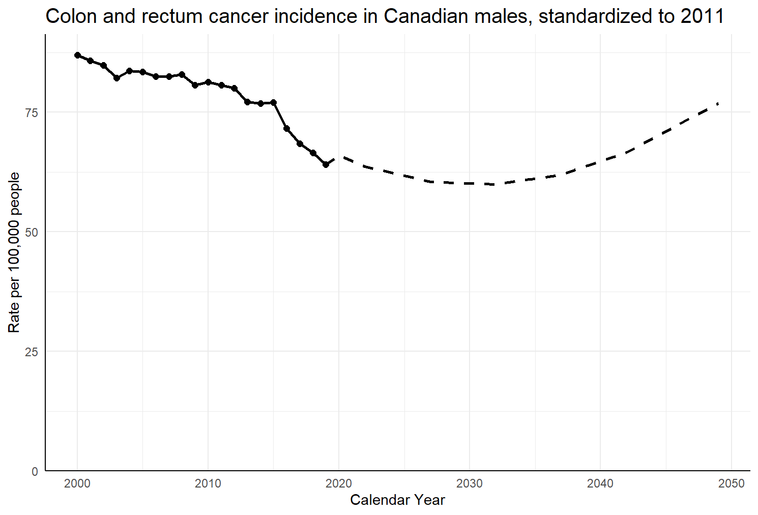
Graph 1: Graph produced by refactored Canproj

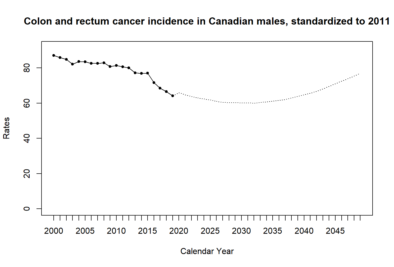
Graph 2: Graph produced by Canproj

Rare cancers and small populations

With sufficiently small case counts, Canproj will select the 5-year average model. During package development, a bug was found that impacts projection results with using both the sum5 = T and sum5 = F methods. The package would calculate rates based on past 6 years instead of 5, occasionally resulting in non-zero projections despite the most recent 5 years of observed data having zero cases.

This example will use the following simulated data.

set.seed(83765)
incidence <- matrix(floor(abs(rnorm(285, 0.1, 0.5))), nrow = 19, ncol = 15)

set.seed(62743)
population <- matrix(floor(rnorm(380, 50000, 750)), nrow = 19, ncol = 20)

# Commands used to run Canproj:
canproj(incidence, population, 2025, stdpop_Canada_2011)
canproj(incidence, population, 2025)

The bug has been fixed in the refactored package, resulting in different projections across packages.

Refactored Canproj
	asr	case
2019	0.409781	3
2020	0.122117	2
2021	0.301660	3
2022	0.129736	1
2023	0.106271	1
2024	0.110790	1
2025	0.154606	2
2026	0.154606	2
2027	0.154606	2
2028	0.154606	2
2029	0.154606	2

Canproj
	asr	case
2019	0.409781	3
2020	0.122117	2
2021	0.301660	3
2022	0.129736	1
2023	0.106271	1
2024	0.110790	1
2025	0.196576	2
2026	0.196576	2
2027	0.196576	2
2028	0.196576	2
2029	0.196576	2

In this case, the refactored package produces slightly lower projections than the original Canproj. Refactored Canproj uses the most recent 5 observed years (2020-2024) to calculate averages, while Canproj projected inflated rates due to including 2019 during calculations.

Male oral cancer incidence in Manitoba

Canproj occasionally projects extreme and absurd growth in cases. In such cases, the error is not caused by model selection but happens due to the way model fitting and projection are performed. The refactored package includes a simply sanity check to try and identify when the error occurs.

This is done by calculating two annual percent changes (APCs): one for all observed years, and one for all projected years. If the difference between APCs is greater than 10, a warning message is produced to alert the user.

This example uses male oral cancer in Manitoba. Canproj projections show a stark difference between observed and projected periods, where observed cases hover around 110 people per year, but projected cases reach into the 4000s. The difference in APCs is about 15%, triggering the console warning.

library(canproj)
  
incidence <- canproj::oral_incidence_mb

population <- canproj::mb_male_population

weights <- c(
  stdpop_Canada_2011@weights[1:17], 
  stdpop_Canada_2011@weights[18] + stdpop_Canada_2011@weights[19])
standpop <- StandardPopulation(
  name = "18grp Canada 2011", 
  strata = as.character(1:18), 
  weights = weights)

proj_oral_incidence_mb <- canproj(incidence, population, 2013, standpop)

Observed incidence
	asr	case
1983	38.99120	140
1984	42.49274	125
1985	40.34210	110
1986	31.08622	75
1987	49.68029	105
1988	57.59196	115
1989	52.24650	105
1990	50.92883	120
1991	41.78482	80
1992	46.14897	115
1993	53.34537	80
1994	38.59026	115
1995	28.59909	75
1996	26.18000	130
1997	34.63679	110
1998	35.10166	115
1999	23.92101	100
2000	29.61766	100
2001	12.46778	75
2002	29.10058	140
2003	27.72893	110
2004	22.64566	80
2005	30.81030	95
2006	45.21595	125
2007	35.35092	110
2008	38.11840	105
2009	43.37524	110
2010	22.47288	85
2011	44.42704	165
2012	31.25867	120

Projected incidence
	asr	case
2013	32.51331	150
2014	29.95657	170
2015	27.39101	199
2016	27.91999	240
2017	31.47670	296
2018	42.19348	371
2019	60.63580	465
2020	76.94678	583
2021	100.11654	723
2022	132.16525	888
2023	168.52045	1072
2024	202.54049	1285
2025	228.37219	1523
2026	234.52375	1780
2027	252.07314	2057
2028	291.15289	2360
2029	109.22680	2674
2030	141.64001	2989
2031	190.88996	3309
2032	238.77524	3602
2033	289.46234	3884
2034	368.35046	4126
2035	495.10752	4351
2036	578.07376	4548
2037	687.43069	4730
2038	729.67026	4896